Using trac to build tree-aggregated predictive models
Source: vignettes/trac-example.Rmd
trac-example.RmdIn this vignette, we demonstrate the basic usage of the trac package, which implements the methodology from Tree-Aggregated Predictive Modeling of Microbiome Data. We use the Gut (HIV) data set, one of the main examples in the paper, which is included in the trac package as sCD14. For more on this data set, see ?sCD14.
The trac package assumes that you want to predict some response variable based on amplicon data1, where the amplicons are structured on a tree.
To apply trac, one needs three things:
A response vector
yof lengthn, wherenis the number of samples.A
n-by-pdata matrixx, wherepis the number of leaves (i.e., the number of taxa at the base level, which in this example is the OTU level).A binary matrix
Awithprows and a column for each non-root node of the tree. In particular, elementA[j,u]indicates whether leafjhas ancestoru.
A look at the sCD14 data object reveals that it has these three elements in addition to two other objects:
The object tree is of class phylo and is useful for plotting. The object of class tax is convenient for seeing the ancestor taxa of a leaf.
If you are starting with a phyloseq object, you can use the functions tax_table_to_phylo and phylo_to_A to form the tree and A objects. See here for a demonstration of this workflow (which describes details of how to handle unclassified taxa and data sets with multiple kingdoms).
Set up train/test splits and take logarithm
Let’s start by splitting the data into a train and test set. We’ll take 2/3 of the observations for training.
Since trac operates in the log-contrast framework, we take the log of the feature matrix.
log_pseudo <- function(x, pseudo_count = 1) log(x + pseudo_count)
ytr <- sCD14$y[tr]
yte <- sCD14$y[-tr]
ztr <- log_pseudo(sCD14$x[tr, ])
zte <- log_pseudo(sCD14$x[-tr, ])
Apply trac
We now solve the trac optimization problem using a path algorithm (implemented in the c-lasso Python package). The function trac returns the solutions for a grid of values of the tuning parameter \(\lambda\). The grid’s minimal value and number of points are controlled by min_frac and nlam, respectively.
fit <- trac(ztr, ytr, A = sCD14$A, min_frac = 1e-2, nlam = 30)By default, trac gives us the model known as “trac (a=1)” in the paper. For other choices of weights, see the section on weights below.
Looking at the trac output
We can look at the trac regularization path. By default, the function plot_trac_path shows the alpha coefficients.
plot_trac_path(fit)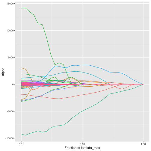
plot of chunk plot_trac_path_alpha
There is an alpha coefficient corresponding to each node of the tree. For example, early in the path we have the following:
show_nonzeros <- function(x) x[x != 0]
show_nonzeros(fit[[1]]$alpha[, 2])
#> Life::Bacteria::Firmicutes::Clostridia::Clostridiales::Ruminococcaceae
#>                                                               306.4128
#> Life::Bacteria::Firmicutes::Clostridia::Clostridiales::Lachnospiraceae
#>                                                              -306.4128
We can also plot the beta values (coefficients corresponding to the leaf taxa):
plot_trac_path(fit, coef = "beta")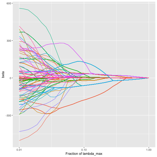
plot of chunk plot_trac_path_beta
We see that as the amount of regularization increases, the individual beta coefficients tend to fuse together (corresponding to the aggregation of taxa induced by the trac regularizer).
Next, we would like to select a value of the tuning parameter. We do so using cross validation.
Cross validate trac to choose tuning parameter
The function cv_trac by default performs 5-fold cross validation.
cvfit <- cv_trac(fit, Z = ztr, y = ytr, A = sCD14$A)
#> fold 1
#> fold 2
#> fold 3
#> fold 4
#> fold 5
We can use the function plot_cv_trac to visualize.
plot_cv_trac(cvfit)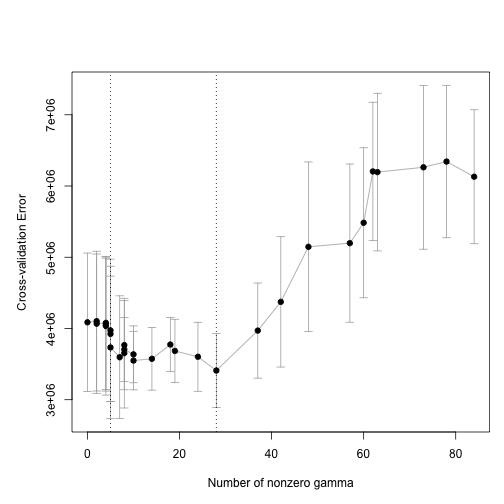
plot of chunk plot_cv
The two vertical lines show us the minimum of the CV curve and the “1 SE rule” solution.
cvfit$cv[[1]]$ibest
#> [1] 20
cvfit$cv[[1]]$i1se
#> [1] 8
Using the 1SE rule results in the following nonzero alpha coefficients.
show_nonzeros(fit[[1]]$alpha[, cvfit$cv[[1]]$i1se])
#>                                                         Life::Bacteria::Actinobacteria
#>                                                                              -501.4344
#> Life::Bacteria::Bacteroidetes::Bacteroidia::Bacteroidales::Bacteroidaceae::Bacteroides
#>                                                                               286.8039
#>                 Life::Bacteria::Firmicutes::Clostridia::Clostridiales::Ruminococcaceae
#>                                                                              2221.7521
#>                 Life::Bacteria::Firmicutes::Clostridia::Clostridiales::Lachnospiraceae
#>                                                                             -1644.8563
#>                                                                         Life::Bacteria
#>                                                                              -362.2653
Making predictions
We can apply our trac model to make predictions on the test set and compute the mean squared error on the test set.
yhat_te <- predict_trac(fit, new_Z = zte)
testerr <- colMeans((yhat_te[[1]] - yte)^2)
nnz <- colSums(fit[[1]]$alpha != 0)
And we can make a plot of the test error as a function of the number of non-zero alpha coefficients.
library(tidyverse)
tibble(nnz = nnz, testerr = testerr) %>%
  ggplot(aes(x = nnz, y = testerr)) +
  geom_point() +
  geom_vline(xintercept = nnz[cvfit$cv[[1]]$i1se])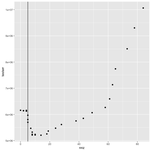
plot of chunk plot_trac_testerr
Weights
The user can specify any set of node-specific weights in the penalty. As described in the trac paper, a straightforward choice is to take a power of the number of leaves under that node:
\[
w_u=|L_u|^{-a}.
\] With apologies to the user, the weights notation is overloaded, which means that the notation w in the function trac and the \(w\) referred to in the paper are different from each other in a way we explain now. In the package, the weights w refer to the weights on the trac optimization problem parameterized in terms of gamma whereas in the paper’s equation (2), \(w\) refers to the weights on the trac optimization problem parameterized in terms of alpha. As explained in the appendix of the paper, \(\alpha_u=\gamma_u\cdot|L_u|\). This means that the weights we use in the package should be taken to be |L_u| times larger than what they are in the paper.
Thus, when the paper writes “trac (a=1)”, this corresponds to the trac function getting an input w of all ones (which is the default). When the paper writes “trac (a=1/2)”, this corresponds to the trac function called as follows:
Other base levels
The trac package can perform its flexible and data-adaptive aggregation starting from any base level of aggregation. In the above, we started with OTU-level data on the leaves of the tree. However, some users may prefer to first aggregate to a fixed level by summing all counts within a certain taxonomic level. For example, we could start by aggregating to the family level before applying trac:
sCD14_family <- aggregate_to_level(sCD14$x, sCD14$y, sCD14$A, sCD14$tax, level = 6, collapse = TRUE)We can now proceed as before
fit_family <- trac(log_pseudo(sCD14_family$x[tr, ]),
                   sCD14_family$y[tr],
                   sCD14_family$A,
                   min_frac = 1e-2, nlam = 30)
Sparse Log-Contrast
One can also fit sparse log-contrast models in trac.
fit_slc <- sparse_log_contrast(ztr, ytr, min_frac = 1e-2, nlam = 30)
cvfit_slc <- cv_sparse_log_contrast(fit_slc, Z = ztr, y = ytr)
#> fold 1
#> fold 2
#> fold 3
#> fold 4
#> fold 5
yhat_te_slc <- predict_trac(list(fit_slc), new_Z = zte)[[1]]
testerr_slc <- colMeans((yhat_te_slc - yte)^2)
nnz_slc <- colSums(fit_slc$beta != 0)
tibble(nnz = nnz_slc, testerr = testerr_slc) %>%
  ggplot(aes(x = nnz, y = testerr)) +
  geom_point() +
  geom_vline(xintercept = nnz[cvfit$cv[[1]]$i1se])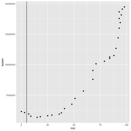
plot of chunk plot_slc_testerr
or more generally any kind of compositional data↩︎